Future-facing conservation units for the Yosemite toad
Tutorial · Landscape genomics in R
Future-facing conservation units for the Yosemite toad
A hands-on walk through the analysis in Maier et al. (2023, Evolutionary Applications): find loci responding to climate, model them with Gradient Forests, map where populations would need to change most by late century, and group meadows into Geminate Evolutionary Units.
Why look forward when drawing conservation units?
Conservation units are usually drawn from the past. Evolutionarily Significant Units (ESUs) capture lineages that diverged long ago, and Management Units (MUs) capture gene pools that are demographically independent today. Both are useful, but managers mostly want to know what will persist. Under rapid climate change, the populations that matter most may be the ones whose adaptive variation fits the conditions coming next, and those need not line up with ancient lineage boundaries.
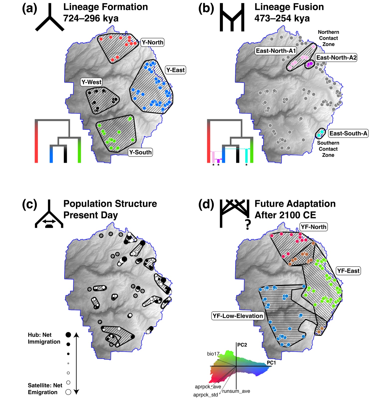
In the paper we proposed Geminate Evolutionary Units (GEUs): groups of populations that share an adaptive response to the environment and so may seed future lineages. The name borrows from geminate species, pairs that diverge after a barrier splits them, because that is what these units are positioned to become. The full framework places ESUs, MUs, and GEUs on one timeline, from lineage formation in the ancient past to adaptation and persistence in the near future.
The Yosemite toad (Anaxyrus canorus) is a good test case. It is federally threatened, it breeds in shallow snowmelt pools in high Sierra meadows, and its whole life cycle is tied to snowpack and runoff. It also has a well-studied history: seven lineages in Yosemite National Park, including admixed populations in contact zones (Maier et al. 2019).
Each time frame calls for its own kind of unit, and the toad has been studied in each one. The figure and table below set them side by side, with links to the papers and to the research page where each is discussed.
 Ancient past |
 More recent past |
 Present |
 Near future |
|
|---|---|---|---|---|
| Process | I. Lineage isolation II. Lineage adaptation |
Secondary contact with admixture and introgression | Demographically independent populations | Future adaptation and population persistence |
| Evolutionary forces | I. Drift–mutation balance II. Divergent selection |
Outbreeding, hybrid vigor, and recombination | Drift–migration balance | Hard and soft selection |
| Genetic pattern | I. Fixed alleles or reciprocal monophyly II. Non-exchangeability |
High genome-wide π, high heterozygosity between populations, and unique alleles | Distinct gene pools with dispersal rates below 10% | Outlier alleles correlated with future environmental gradients |
| Unit | ESUs | GEUs (in contact zones) | MUs (can be hierarchical) | GEUs |
| In the Yosemite toad | Maier et al. 2019 Research page |
Maier et al. 2019 (fused lineages) Maier et al. 2024 (adaptive introgression) Research page · islands and rivers |
Maier et al. 2022 Research page |
Maier et al. 2023 (this tutorial) Research page |
Each step below shows the main pieces of code. The complete scripts are in the code download. Steps that take hours (bayenv2, hyperparameter tuning, the Geonomics simulations) are shown and then read from saved results.
Data and setup
The inputs are on Dryad at doi:10.5061/dryad.6m905qg3r: SNP allele counts for 102 meadows (90 in Yosemite and 12 in Kings Canyon), climate at each meadow, bayenv2 output, and current and future climate rasters. Unzip it as YOTOAD_CLIMATE_ADAPTATION/. The data bundle adds one small file, scaling.csv, described in step 1.
About locations. The Yosemite toad is federally threatened, so the archive leaves out meadow coordinates. Everything in this tutorial runs from the archive and the data bundle. Maps show the whole park and never plot sampled meadows.
The code uses current packages, with terra and sf in place of raster and rgdal. Gradient Forests is not on CRAN; install it from R-Forge. It was tested on R 4.5.3.
install.packages(c("dplyr", "tidyr", "sf", "terra", "vegan", "cluster",
                   "ggplot2", "patchwork", "ggnewscale", "ggrepel"))
install.packages(c("extendedForest", "gradientForest"),
                 repos = "https://R-Forge.R-project.org", type = "source")
DATA_DIR <- "path/to/YOTOAD_CLIMATE_ADAPTATION"
Step 1. Climate today and in the future
We used 30 variables known to matter for Yosemite toads: the 19 WorldClim bioclimatic variables (1 km) and 11 hydrological variables from the California Basin Characterization Model (BCM, 270 m), such as April 1 snowpack, runoff, recharge, and climatic water deficit. Current climate is 1960–1990 (WorldClim) and 1981–2010 (BCM). Future climate comes from CCSM4 under RCP 8.5, a business-as-usual scenario, for 2061–2080 (WorldClim) and 2070–2099 (BCM). Every layer is resampled to a 90 m elevation grid.
elev <- rast(file.path(DATA_DIR, "rasters", "current_env_noclip", "elevation.tif"))
stack_clim <- function(files) {
  s <- rast(lapply(files, function(f) resample(rast(f), elev, method = "bilinear")))
  mask(s, yosemite_boundary)
}
cur <- stack_clim(current_files)   # 19 bio_*.tif plus 11 BCM layers
fut <- stack_clim(future_files)
The archive stores climate at each meadow centered and scaled across the 102 meadows (toad.env.pca.data.txt, one row per variable). A model fit on those values has to predict pixels on the same scale, so the data bundle includes the mean and standard deviation of each variable. With them, every pixel goes onto the meadow scale in one line.
scaling <- read.csv("scaling.csv")
pix_cur <- as.data.frame(cur, xy = TRUE, cells = TRUE, na.rm = TRUE)
for (v in scaling$variable) {
  pix_cur[[v]] <- (pix_cur[[v]] - scaling$mean[scaling$variable == v]) / scaling$sd[scaling$variable == v]
}
That gives 446,375 pixels across Yosemite, each with present and future climate.
Step 2. Finding loci that respond to climate
The genetic data are 2,039 SNPs (one per ddRADseq locus) from 102 meadows. Kings Canyon meadows were included at this step only, as an outgroup, to raise confidence that a candidate reflects climate and not one lineage’s history. Population structure is the big trap in genotype-environment association: lineages differ in allele frequency and also live in different climates. We used two methods that handle it differently, and kept only loci that both flagged.
The first is a partial redundancy analysis (RDA). Allele frequencies are regressed on climate (the first five principal components of the 30 variables), latitude, longitude, and elevation. Population structure (five PCs of the allele frequencies) and spatial autocorrelation (four Moran’s eigenvector maps) are partialled out first. Loci with loadings more than two standard deviations from the mean on any significant axis are candidates.
library(vegan)
pca_pop <- prcomp(freq, center = TRUE, scale. = TRUE)          # population structure
d <- data.frame(env, pca_pop$x[, 1:5])
rda_fit <- rda(freq ~ PC1 + PC2 + PC3 + PC4 + PC5 + long + lat + elevation +
                 Condition(PC1.pop + PC2.pop + PC3.pop + PC4.pop + PC5.pop +
                           MEM1 + MEM2 + MEM3 + MEM4),
               data = d, scale = TRUE)
load <- scores(rda_fit, choices = 1:4, display = "species")    # axes 1-4 were significant
z <- apply(load, 2, function(x) abs(x - mean(x)) / sd(x))
rda_candidates <- rownames(z)[apply(z > 2, 1, any)]
The second is bayenv2, which estimates a covariance matrix of allele frequencies among meadows (shared ancestry) and then tests each SNP against each variable with that structure accounted for. We ran it ten times and averaged. A SNP is a candidate if its Bayes factor is in the top 2.5% and its Spearman correlation in the top 5% for at least one variable. Candidates tied to the spatial eigenvector maps were dropped, since those most likely reflect population history.
runs <- lapply(1:10, function(i) read.table(file.path(DATA_DIR, "bayenv2", paste0("out", i, ".txt")))[, 2:37])
be <- Reduce(`+`, lapply(runs, as.matrix)) / 10
bf <- be[, seq(1, 36, 3)]; rho <- be[, seq(2, 36, 3)]
hit <- bf > quantile(bf, 0.975) & abs(rho) > quantile(abs(rho), 0.95)
bayenv_candidates <- loci[rowSums(hit[, climate_cols]) > 0 & rowSums(hit[, mem_cols]) == 0]
In the paper the RDA gave 394 candidates and bayenv2 gave 70, and 24 SNPs were in both. A rerun from the archived files with current package versions gives back the same 70 bayenv2 candidates. The RDA list depends on fine details of the allele frequency table, and a rerun gives 429 candidates, 15 of them shared with bayenv2. The published list of 24 is in Table S4 of the paper, and the rest of this tutorial uses it so every later step matches the paper.
outliers <- c("I61882", "I71263", "I67875", "I28646", "I54027", "I49572", "I31252", "I36117",
              "I44097", "I55572", "I50736", "I25880", "I32153", "I18477", "I57671", "I49074",
              "I43560", "I31700", "I41319", "I3403",  "I6634",  "I24442", "I43270", "I49871")
Step 3. Gradient Forests
Gradient Forests (Ellis et al. 2012) fits a random forest for each SNP, predicting its allele frequency from climate, then pools the split points across all SNPs. The result is a turnover function for every climate variable: how much allele frequencies change, in total, as you move along that gradient. Steep parts of a curve are thresholds where adaptive composition shifts quickly. Because the functions are nonlinear, they capture what a linear association test would miss.
The model is fit to the 90 Yosemite meadows. Hyperparameters were tuned in the paper by ten-fold cross-validation over the number of trees, mtry, maxLevel, and the correlation threshold (Table S5). That takes hours, so here we use the chosen values. For comparison, a second model is fit to 300 randomly chosen SNPs.
library(gradientForest)
set.seed(12345)
ref <- freq_yose[, sample(ncol(freq_yose), 300)]       # reference set
gf_out <- gradientForest(cbind(env_yose, freq_yose[, outliers]),
                         predictor.vars = climate_vars, response.vars = outliers,
                         ntree = 5000, mtry = 8, maxLevel = 2, corr.threshold = 0.5)
gf_out$result                                         # R2 for each SNP the model could fit
importance(gf_out, type = "Weighted")                 # R2-weighted importance of each variable
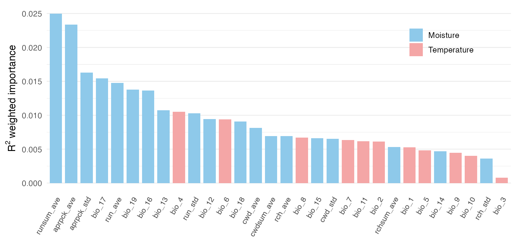
19 of the 24 SNPs have a positive fit (R² above zero), as in the paper, with a mean R² of 0.28 against 0.22 for the random reference set. Adaptive genetic variation tracks moisture much more than temperature. The most important variables are average summer runoff, April 1 snowpack and its variability from year to year, and precipitation in the driest quarter.
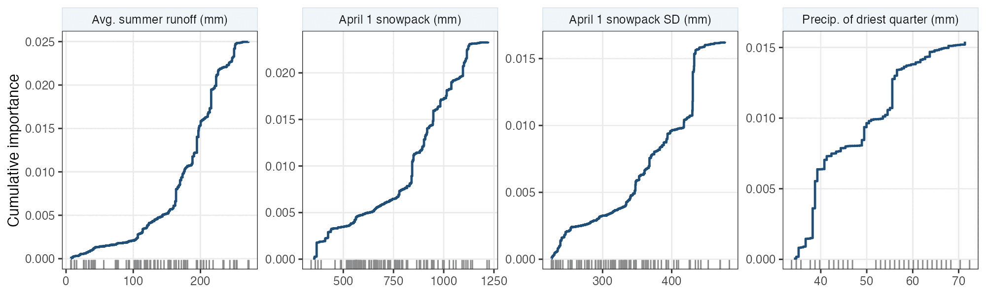
The curves show where along each gradient the change happens. For summer runoff and snowpack, most of the turnover sits at the upper end, among the wettest, snowiest meadows. Small losses of snow at high elevation could therefore mean large changes in which alleles are favored.
Step 4. Mapping adaptation today and the change needed
The fitted model can transform any climate into “genetic space”: each variable is replaced by its position on its cumulative importance curve, so distances between pixels measure expected differences in adaptive allele frequency. Projecting every pixel and coloring the first three principal components (following Fitzpatrick & Keller 2015) gives a map of adaptive composition. Pixels with similar colors are expected to hold similar adaptive variation.
cur_t <- predict(gf_out, pix_cur[, climate_vars])
fut_t <- predict(gf_out, pix_fut[, climate_vars])
pca <- prcomp(cur_t, center = TRUE, scale. = FALSE)
a1 <- -pca$x[, 1]; a2 <- pca$x[, 2]; a3 <- pca$x[, 3]
rgb01 <- function(v) (v - min(v)) / (max(v) - min(v))
colour <- rgb(rgb01(a1 + a2), rgb01(-a2), rgb01(a3 + a2 - a1))
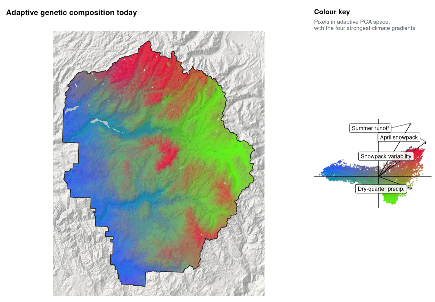
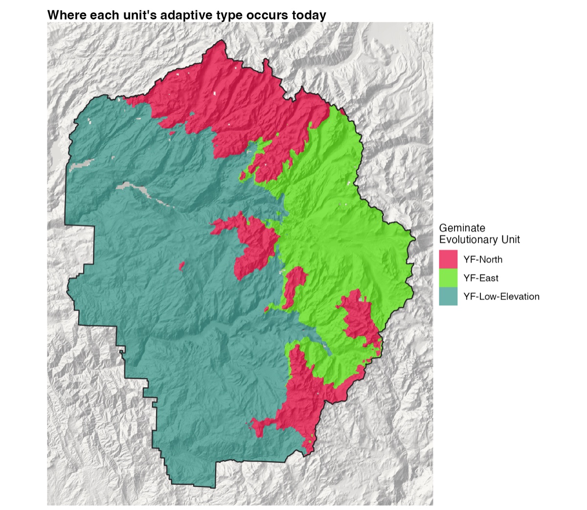
Three broad regions stand out, and they echo the lineage boundaries without matching them exactly. Toads in the north appear adapted to high winter snowpack with moderate summer rain. Toads in the east appear adapted to low to moderate snowpack with high summer rain. Toads at lower elevation in the west and south share a third type, adapted to low snowpack and little rain, even though they come from two different ancestral lineages.
The same transformation applied to future climate shows how far each place moves in genetic space. The distance between a pixel’s present and future positions, often called genetic offset, is the change in allele frequency a population there would need to stay as well adapted as it is now. We wrote it as δ(f).
offset <- sqrt(rowSums((fut_t - cur_t)^2))
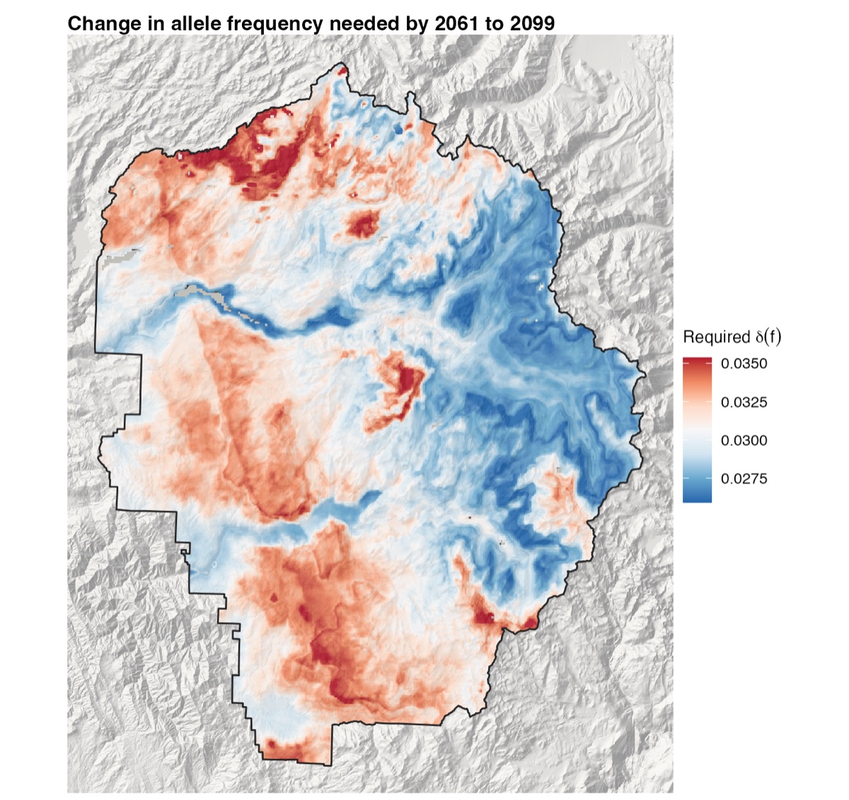
The largest required change falls in the west, the far north, and the south. The high eastern country, home to the Y-East lineage, needs the least. Summer rain is forecast to rise everywhere and most at high elevation, but the turnover curve is shallow at the high end, so the extra rain changes the adaptive optimum there only a little.
Step 5. Geminate Evolutionary Units
To turn a continuous map into units, we predicted the adaptive composition of each of the 90 meadows from its present climate, summarized it with PCA, and clustered meadows with k-means. Both the elbow method and the average silhouette width point to three clusters.
pred <- predict(gf_out, env_yose[, climate_vars])
pca_m <- prcomp(pred, center = TRUE, scale. = FALSE)
wss <- sapply(1:12, function(k) kmeans(pca_m$x, k, nstart = 10)$tot.withinss)
sil <- sapply(2:12, function(k) mean(cluster::silhouette(kmeans(pca_m$x, k, nstart = 10)$cluster,
                                                         dist(pca_m$x))[, 3]))
km <- kmeans(pca_m$x, centers = 3, nstart = 10, iter.max = 1000)
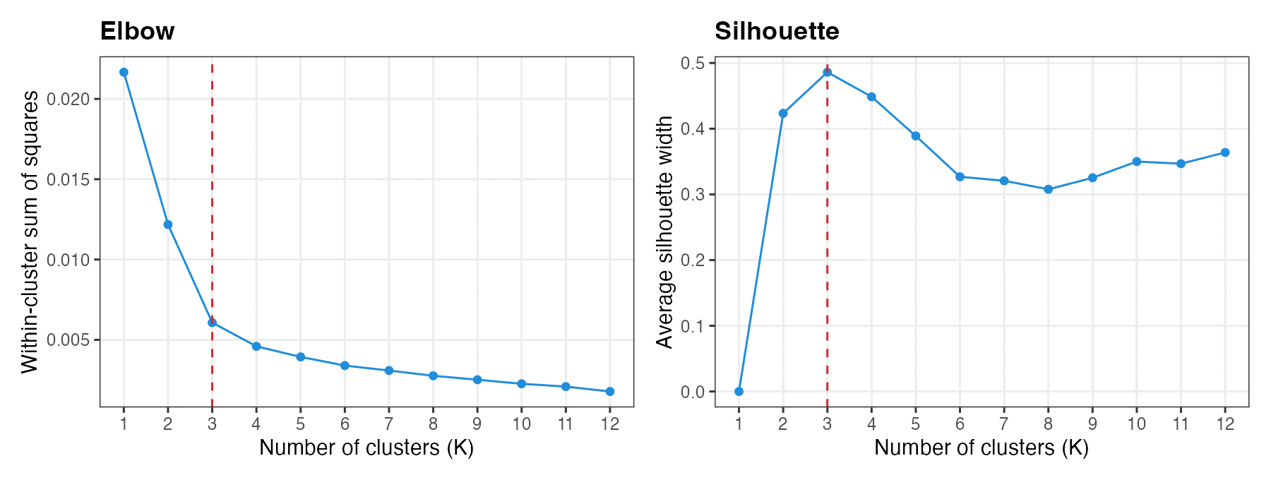
We named the three units after the lineages they mostly hold, with a “YF” prefix for Yosemite future. YF-North combines Y-North and most of the admixed East-North-A1 meadows. YF-East combines Y-East with East-North-A2. YF-Low-Elevation joins the two low-elevation lineages, Y-West and Y-South, which split long ago but now share one adaptive type.
| Ancestral lineage | YF-North | YF-East | YF-Low-Elevation |
|---|---|---|---|
| Y-North | 10 | · | · |
| East-North-A1 | 6 | 1 | · |
| East-North-A2 | · | 3 | · |
| Y-East | 2 | 35 | · |
| East-South-A | 2 | · | · |
| Y-South | 1 | · | 14 |
| Y-West | · | · | 16 |
| Total | 21 | 39 | 30 |
Meadows in the two contact zones did not resolve cleanly into one unit or another (brown in panel d of the timeline figure). In the paper they were assigned to intermediate, overlapping GEUs, because of their mixed clustering and unusually high genome-wide diversity. A zone carrying novel recombinant variation may matter more for future adaptation than its ambiguous membership suggests.
Coloring every pixel by the unit whose center is nearest in adaptive space shows where each adaptive type occurs across the park. The map covers all of Yosemite, including ground toads don’t use, so it is best read as a picture of climate-driven adaptive types rather than of habitat.
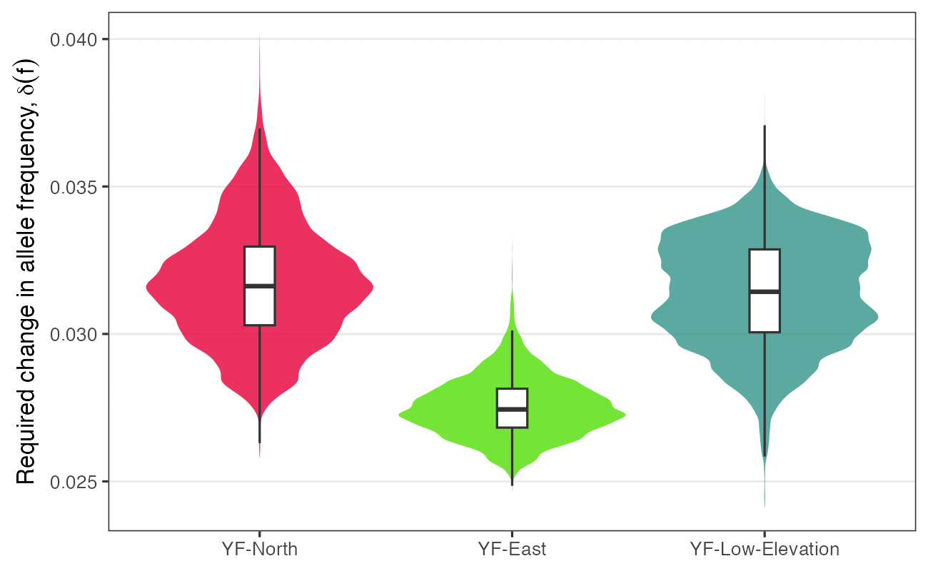
Overlaying the offset map on the units gives each unit’s exposure. YF-East faces clearly less required change (median 0.0274) than YF-North (0.0316) or YF-Low-Elevation (0.0314).
Step 6. Simulating fitness and persistence
Required change says how far a population has to go, but not whether it can get there. That depends on standing variation, population size, and how strongly selection acts. To bring those together we ran spatially explicit, individual-based simulations in Geonomics v1.3.6 (Terasaki Hart et al. 2021). Fitness of individual i follows
ωi = 1 − φx,y |ex,y − zi|γ
where e is the optimal phenotype for the climate at that location, z is the individual’s phenotype, φ is the strength of selection, and γ = 1. The model runs on a 45 × 58 grid of 1.35 km cells covering Yosemite. Three layers drive it:
- Movement. Toads disperse over the migration surface from our corridor work (Maier et al. 2022, Heredity).
- Carrying capacity. Interpolated effective population size (Ne) sets how many toads each cell can hold, scaled to about 30,000 toads in roughly 300 occupied meadows. The strength of selection φ varies with it, since selection works better in larger populations.
- Selection. One layer per year from 2011 to 2100 holds the optimal phenotype: the Gradient Forests prediction of δ(f) from 2010 to that year.
The trait is controlled by the 24 candidate loci. After a burn-in under stable climate, the optimum shifts every simulated year, and the whole run is repeated ten times. The model file and its input layers are on Dryad (geonomics/). Running it looks like this in Python:
# pip install geonomics==1.3.6
import rasterio
import geonomics as gnx
from geonomics.sim.params import _read_params_file

params = _read_params_file("GNX_yotoad_climate_adaptation.py")
phi = rasterio.open("suitability/suitability.tif").read()[0, :, :]   # selection strength by cell
params["comm"]["species"]["canorus"]["gen_arch"]["traits"]["trait_clim"]["phi"] = phi
mod = gnx.make_model(params)
mod.run(verbose = True)   # ten iterations, several hours
Each iteration writes every individual at every time step (location, phenotype, and fitness) to CSV files. Individuals are then grouped by the GEU they fall in and summarized over time. The R code for that step is in ToadClimateAdaptation.R on Dryad, in the section on Geonomics simulations. The full run takes several hours, so the figure below shows the output from the paper.
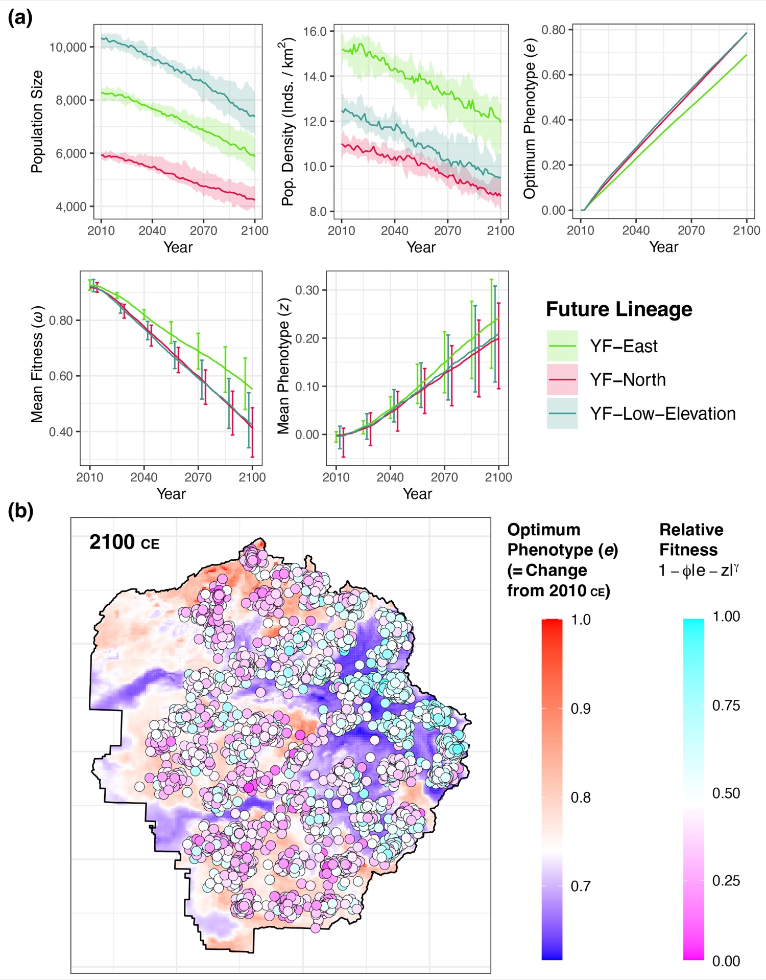
Across ten runs, toads in Yosemite declined by a median of 29% (range 19–36%) over 90 years. YF-Low-Elevation kept the largest population, because it covers twice the area of the other two units. YF-East was the most stable in density, adapted fastest, and kept the highest mean fitness, for two reasons: it is sheltered from the largest climatic changes, and its higher density and standing diversity let selection work more efficiently. The map tells the same story at the scale of individuals: the high eastern country, where the optimum moves least, holds most of the toads that are still well matched to their climate in 2100.
How to read these maps
These maps show where climate change is expected to push adaptive genetic variation hardest, under one climate model and one emissions scenario. They rest on a few assumptions worth keeping in mind. They assume today’s links between alleles and climate reflect local adaptation and will hold in the future. They come from 24 SNPs, a small window onto what is surely a larger genetic basis for climate adaptation. And they leave out things that will matter a great deal for Yosemite toads: dispersal between meadows, plasticity, disease such as chytridiomycosis, and demography. Tests of genetic offsets in simulations and common gardens have found they track fitness best where local adaptation is strong, and less well in climates unlike any seen today. δ(f) is best read as a relative ranking of exposure, useful for comparing units and places, rather than a forecast of decline. The GEUs are best used alongside the ESUs and MUs they complement, and checked against monitoring data as they come in.
Using this workflow for your own species
Nothing here is specific to toads. The approach suits any species with population-level SNP data and good environmental layers. A few things to keep in mind:
- Guard against population structure twice. Requiring agreement between two methods that correct for structure in different ways cuts false positives, at the cost of missing some real signal.
- Use a reference set. Fitting the same model to random SNPs shows how much of the turnover is specific to the candidates.
- Pick variables you can defend. Gradient Forests ranks whatever you give it. Variables tied to the species’ biology (here, snowpack and runoff for a snowmelt breeder) make the results easier to interpret and act on.
- Keep the scale consistent. If meadow values are standardized, pixels must be standardized with the same means and standard deviations before prediction.
- Match units to decisions. Units drawn from future adaptation answer a different question than units drawn from lineage history. Present both.
How to cite
- Maier PA, Vandergast AG, Bohonak AJ (2023) Using landscape genomics to delineate future adaptive potential for climate change in the Yosemite toad (Anaxyrus canorus). Evolutionary Applications 16(1):74–97. doi:10.1111/eva.13511. Data: doi:10.5061/dryad.6m905qg3r
Related work
- Maier PA, Vandergast AG, Ostoja SM, Aguilar A, Bohonak AJ (2022) Landscape genetics of a sub-alpine toad: climate change predicted to induce upward range shifts via asymmetrical migration corridors. Heredity 129:257–272. doi:10.1038/s41437-022-00561-x
- Maier PA, Vandergast AG, Ostoja SM, Aguilar A, Bohonak AJ (2022) Gene pool boundaries for the Yosemite toad (Anaxyrus canorus) reveal asymmetrical migration within meadow neighborhoods. Frontiers in Conservation Science 3:851676. doi:10.3389/fcosc.2022.851676
- Maier PA, Vandergast AG, Ostoja SM, Aguilar A, Bohonak AJ (2019) Pleistocene glacial cycles drove lineage diversification and fusion in the Yosemite toad (Anaxyrus canorus). Evolution 73:2476–2496. doi:10.1111/evo.13868
- Maier PA, Vandergast AG, Bohonak AJ (2024) Yosemite toad (Anaxyrus canorus) transcriptome reveals interplay between speciation genes and adaptive introgression. Molecular Ecology 33(8):e17317. doi:10.1111/mec.17317
- Ellis N, Smith SJ, Pitcher CR (2012) Gradient forests: calculating importance gradients on physical predictors. Ecology 93:156–168.
- Fitzpatrick MC, Keller SR (2015) Ecological genomics meets community-level modelling of biodiversity: mapping the genomic landscape of current and future environmental adaptation. Ecology Letters 18:1–16.
- Günther T, Coop G (2013) Robust identification of local adaptation from allele frequencies. Genetics 195:205–220.
- Forester BR, Lasky JR, Wagner HH, Urban DL (2018) Comparing methods for detecting multilocus adaptation with multivariate genotype–environment associations. Molecular Ecology 27:2215–2233.
- Terasaki Hart DE, Bishop AP, Wang IJ (2021) Geonomics: forward-time, spatially explicit, and arbitrarily complex landscape genomic simulations. Molecular Biology and Evolution 38:4634–4646.