Tutorial · Landscape genetics in R
Migration corridors and climate change forecasts for the Yosemite toad
A hands-on walk through the analysis in Maier et al. (2022, Heredity), from pairwise FST to least cost corridors, Cubist models of connectivity, and maps of where migration is projected to shift by the end of the century.
Why model corridors this way?
The Yosemite toad (Anaxyrus canorus) is a meadow specialist of the high Sierra Nevada. Tadpoles live in ultra-shallow snowmelt pools, so the species depends on snowpack, runoff and spring recharge, which are exactly the things climate change is expected to alter most. Adults forage and disperse through the forest, rock and shrub between meadows. A useful model of connectivity has to treat both: the environment along migration routes, and the contrast between the meadows at either end.
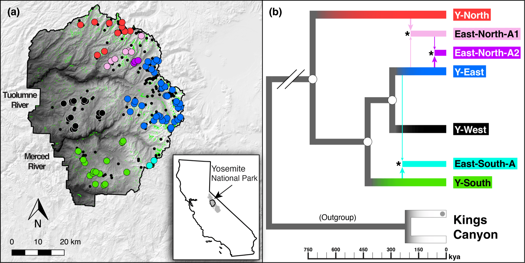
Most landscape genetic studies fold every hypothesis into a single resistance surface. That works for one or two variables, but it gets unwieldy fast, and translating raw values into resistance is somewhat subjective. In the paper we split the problem in two. First we find the most likely migration paths using two features already known to matter, slope and vegetation moisture. Then we pull raw values of dozens of features out of corridors around those paths and let a machine learning model sort out which ones explain genetic differentiation. Because the second step works on raw features, each group of features can even have its own corridor width.
Each step below shows the main pieces of code. The complete scripts are in the code download, and they reproduce the published tables. Where a step takes hours on a full dataset, the tutorial shows the code and then reads the saved result, so you can follow along on a laptop.
Data and setup
You need two downloads. The raw inputs (Stacks FST tables, resistance surfaces, environmental rasters, lineage assignments) are on Dryad at doi:10.5061/dryad.xsj3tx99h. Unzip Corridors.zip, FST_YOSE.zip and ResistanceGA.zip into one folder. The tutorial data bundle adds the pairwise tables that steps 2 and 3 produce: path lengths under every hypothesis, environmental values for every corridor bandwidth, and the at-site contrasts. Unzip it into the same folder. The raw reads are on the NCBI SRA under BioProject PRJNA558546.
About locations. The Yosemite toad is federally threatened, so the archive leaves out meadow coordinates. Step 1, the path ranking in step 2, and steps 4 and 5 run from the downloads alone. Building paths and corridors (steps 2 and 3) and mapping the forecasts (step 6) need meadow locations, which qualified researchers can request from the corresponding author. You can also point the same code at your own sites. Every map on this page shows the park as a whole, with meadow symbols displaced by up to 1 km, as in the paper.
The code uses current packages, with sf and terra in place of the retired rgdal, rgeos and maptools. It was tested on R 4.5.3.
install.packages(c("dplyr", "tidyr", "sf", "terra", "gdistance", "exactextractr",
                   "lme4", "MuMIn", "caret", "ranger", "Cubist", "spatialRF",
                   "igraph", "ggplot2", "patchwork", "ggnewscale", "scico", "doParallel"))
DATA_DIR  <- "path/to/unzipped/dryad"          # holds Corridors/, FST_YOSE/, ResistanceGA/
CORR_DIR  <- file.path(DATA_DIR, "Corridors")
MODEL_DIR <- file.path(CORR_DIR, "models2", "SlopeVeg_90_10_")
Step 1. Genetic differentiation and the direction of migration
The genetic data are ddRADseq haplotypes for 535 tadpoles from 90 meadows (2,318 polymorphic loci), processed in Stacks. For every pair of meadows, Stacks wrote a table with one row per SNP. Pairwise FST is the sample-size weighted variance in allele frequency between the two meadows, averaged over SNPs. SNPs whose frequencies do not differ (Fisher’s exact test, P ≥ 0.05) count as zero.
snp_fst <- function(file) {
  d <- read.delim(file, check.names = FALSE)
  p <- cbind(d$p_1_freq, d$p_2_freq)            # allele frequency in each meadow
  n <- cbind(d$n_1, d$n_2)                      # sample sizes
  pbar <- rowSums(p * n) / rowSums(n)
  w <- 2 * n / rowSums(n)
  fst <- rowSums(w * (p - pbar)^2) / (2 * pbar * (1 - pbar))
  fst[d$`Fisher's P` >= 0.05] <- 0
  mean(fst)
}
files <- list.files(file.path(DATA_DIR, "FST_YOSE", "Combined", "fst"),
                    pattern = "^batch_1\\.fst_M[0-9]+-M[0-9]+\\.tsv$", full.names = TRUE)
fst <- parallel::mclapply(files, snp_fst, mc.cores = 8)
Run over all 4,005 pairs, this matches the archived Fst.txt to within 5 × 10⁻¹⁰, which is just rounding.
Differentiation alone has no direction. To capture asymmetry we use directional GST (Sundqvist et al. 2016), which compares each meadow with a hypothetical gene pool shared by the pair. The difference between emigration and immigration gives a relative term, δM. Positive values mean a meadow sends out more migrants than it receives. Working with the difference avoids estimating any explicit migration rate and leans less on island model assumptions such as drift–migration equilibrium. The estimates come from our earlier study of gene pool boundaries (Maier et al. 2022, Frontiers in Conservation Science) and are stored in Fst.txt as gst_out and gst_in.
gen <- read.delim(file.path(CORR_DIR, "fst", "Fst.txt")) |>
  transmute(a = pmin(pop1, pop2), b = pmax(pop1, pop2),   # smaller meadow ID first
            fst = fst_wc.mean, dM = gst_out - gst_in) |>
  rename(pop1 = a, pop2 = b)
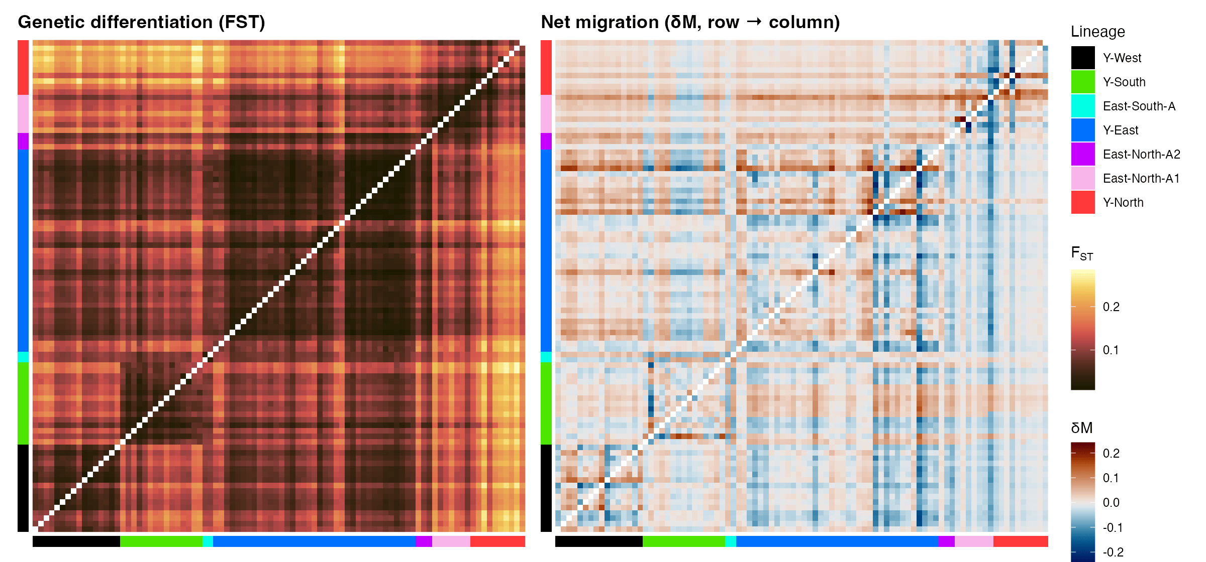
Step 2. Choosing the most likely migration paths
Topographic complexity and moisture are already known to shape Yosemite toad connectivity, so we built path hypotheses from those two features. ResistanceGA (Peterman 2018) optimized a resistance transformation for each one at 300 m, using a genetic algorithm to maximize the fit of mixed models between FST and resistance distance. Both came out as inverse-reverse monomolecular curves. Slope resistance rises gently, so a 30° slope still costs under 2,000, but there is a sharp inflection near 70°. That matches what we see in the field: toads climb moderately steep drainages but seldom breed in meadows cut off by very steep terrain. Steep ridgetops were scored as impassable.
# ResistanceGA (not run here; it takes days). See ResistanceGA/ResistanceGA.R on Dryad.
GA.inputs <- GA.prep(ASCII.dir = "Resistance/", Results.dir = "Results/", select.trans = "M",
                     max.cont = 1e6, cont.shape = "increase", seed = 12345, maxiter = 50, run = 10)
gdist.inputs <- gdist.prep(n.Pops = 90, samples = meadow_points, response = fst_vector,
                           method = "costDistance", directions = 8,
                           transitionFunction = function(x) 1 / mean(x))
result <- SS_optim(gdist.inputs = gdist.inputs, GA.inputs = GA.inputs)
The optimized slope and vegetation surfaces were rescaled, blended in proportions from 0:100 to 100:0, and saved at 30 m in Corridors/resistance2/30m. That gives eleven path hypotheses, plus straight-line distance as the null.
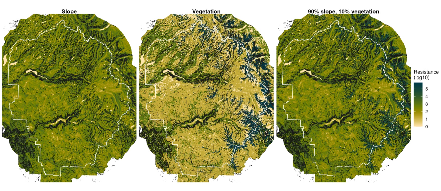
For each blend, gdistance builds a transition layer. Barrier cells are set to NA so no path can cross them, and conductance between neighboring cells is the inverse of their mean resistance. Path length is measured over the terrain surface, not on the flat map.
library(gdistance)
r <- raster::raster(file.path(CORR_DIR, "resistance2", "30m", "SlopeVeg_90_10_30m.tif"))
r[r >= 1e6] <- NA                                    # ridgelines
tr <- transition(r, function(x) 1 / mean(x), directions = 8)
tr <- geoCorrection(tr, type = "c")                  # about a minute for the whole park
path <- shortestPath(tr, xy["359", ], xy["1543", ], output = "SpatialLines") |>
  sf::st_as_sf()
surface_length <- function(line, dem) {              # 3D length along the DEM
  co <- sf::st_coordinates(line)[, 1:2]
  z  <- terra::extract(dem, co)[, 1]
  sum(sqrt(diff(co[, 1])^2 + diff(co[, 2])^2 + diff(z)^2))
}
As a check, the path between meadows 359 and 1543 rebuilt this way is 27,257.2 m long, the same as the archived value. The archive holds path lengths for every pair under every blend, so ranking the hypotheses is quick. We kept pairs whose shortest path is under 30 km, since earlier work found no isolation by distance beyond that scale. For each blend we fit a mixed model of FST on path length, with source and destination meadow as random effects.
library(lme4); library(MuMIn)
fit_one <- function(m) {
  fit <- lmer(as.formula(paste0("fst ~ ", m, " + (1 | From) + (1 | To)")), data = dd)
  r2  <- r.squaredGLMM(fit)
  tibble(Model = m, R2m = r2[, "R2m"], R2c = r2[, "R2c"], AIC = AIC(fit),
         AICc = AICc(fit), BIC = BIC(fit), LL = as.numeric(logLik(fit)))
}
rank_tab <- bind_rows(lapply(models, fit_one)) |> arrange(desc(LL))
| Slope | Vegetation | R²m | R²c | AIC | AICc | BIC | log L |
|---|---|---|---|---|---|---|---|
| 0.9 | 0.1 | 0.104 | 0.912 | −6,176.878 | −6,176.823 | −6,151.904 | 3,093.439 |
| 0.8 | 0.2 | 0.102 | 0.911 | −6,163.112 | −6,163.056 | −6,138.137 | 3,086.556 |
| 0.4 | 0.6 | 0.100 | 0.912 | −6,159.875 | −6,159.820 | −6,134.901 | 3,084.938 |
| 0.5 | 0.5 | 0.098 | 0.911 | −6,152.689 | −6,152.634 | −6,127.715 | 3,081.345 |
| 1 | 0 | 0.090 | 0.910 | −6,143.724 | −6,143.668 | −6,118.749 | 3,076.862 |
| 0.7 | 0.3 | 0.097 | 0.910 | −6,143.199 | −6,143.144 | −6,118.225 | 3,076.600 |
| 0.6 | 0.4 | 0.096 | 0.910 | −6,139.191 | −6,139.136 | −6,114.217 | 3,074.596 |
| 0.3 | 0.7 | 0.094 | 0.910 | −6,138.701 | −6,138.646 | −6,113.727 | 3,074.350 |
| 0.2 | 0.8 | 0.093 | 0.910 | −6,135.075 | −6,135.020 | −6,110.101 | 3,072.538 |
| 0 | 1 | 0.103 | 0.908 | −6,126.692 | −6,126.637 | −6,101.718 | 3,068.346 |
| 0.1 | 0.9 | 0.096 | 0.905 | −6,119.832 | −6,119.777 | −6,094.858 | 3,064.916 |
| None | None | 0.086 | 0.904 | −6,101.830 | −6,101.775 | −6,076.856 | 3,055.915 |
The 90% slope, 10% vegetation model ranks first on log likelihood, AIC and marginal R², and the runner-up also leans on slope (80%). Every path model beats straight-line distance. Because ridgelines bisect the park, this model finds only one route linking each low-elevation lineage (Y-South, Y-West) to the high-elevation Y-East lineage.
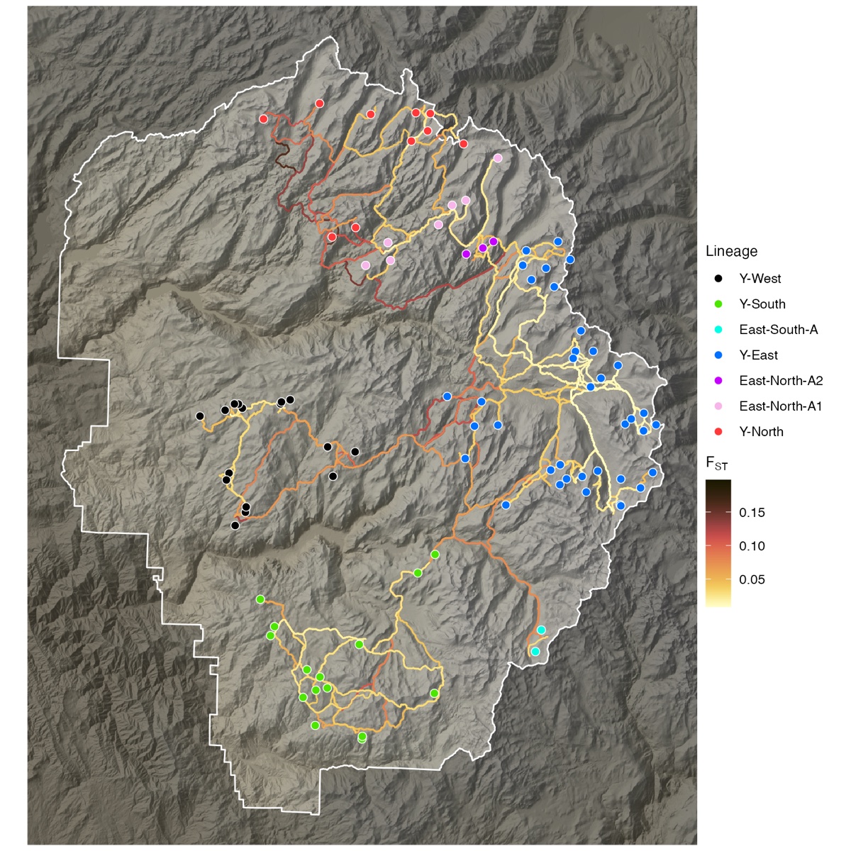
Step 3. From a single path to a corridor
A toad does not walk a one-pixel line, and there are usually several routes of similar cost. So rather than extract environment along the least cost path alone, we tried six corridor bandwidths around it. Two are simple buffers of 100 m and 500 m, chosen around the mean yearly dispersal distance of about 275 m. The other four are least cost corridors. For a pair of meadows, we sum the accumulated cost surfaces from each one; cells with low totals lie on cheap routes between them. We keep the cheapest 0.1%, 0.5%, 1% or 5% of cells and rescale them so the best route has a weight of 1 and the corridor edge a weight of 0. Those weights then decide how much each cell’s environment counts.
acc_cost <- function(id) {
  a <- terra::rast(accCost(tr, xy[as.character(id), , drop = FALSE]))
  a[is.infinite(a)] <- NA
  a
}
lcc <- function(acc_i, acc_j, q) {
  s <- acc_i + acc_j
  rng <- minmax(s)
  s <- (s - rng[1]) / (rng[2] - rng[1])
  v <- sort(values(s, na.rm = TRUE))
  s[s > v[round(length(v) * q)]] <- NA         # keep the cheapest q share of cells
  1 - s / max(values(s), na.rm = TRUE)          # weight 1 on the best route, 0 at the edge
}
acc_i <- acc_cost(359); acc_j <- acc_cost(1543)
lccs <- rast(lapply(c(0.001, 0.005, 0.01, 0.05), \(q) lcc(acc_i, acc_j, q)))
buffers <- lapply(c(100, 500), \(w) sf::st_buffer(path, w))
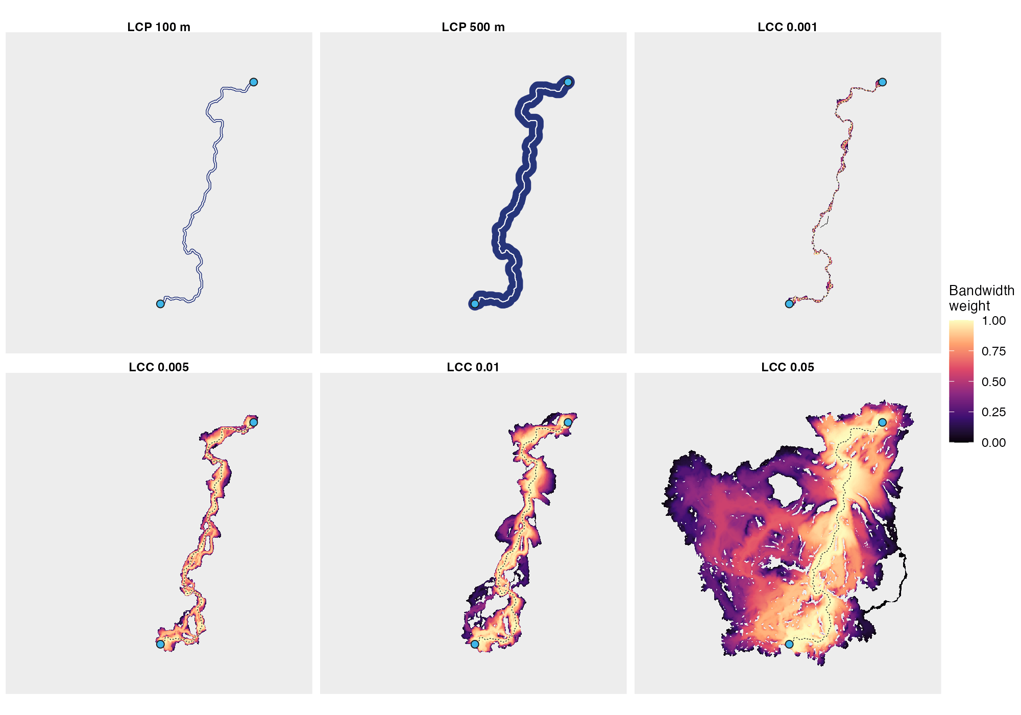
Next, environmental features are summarized inside each corridor. The archive includes 18 climate layers from the California Basin Characterization Model (present and 2070–2099 under CCSM4 RCP 8.5), LANDSAT soil moisture, MODIS snowmelt timing, soil age, topography, vegetation, fire frequency, and trail and road crossings weighted by use. For buffers we take an exact, coverage-weighted mean with exactextractr. For corridors we resample each layer to the 30 m corridor grid and weight every cell by its corridor weight.
corridor_mean <- function(env, w) {
  env <- resample(env, w, method = "bilinear")
  global(env * w, "sum", na.rm = TRUE)[[1]] / global(w, "sum", na.rm = TRUE)[[1]]
}
buffer_mean <- function(env, poly) {
  x <- exactextractr::exact_extract(env, poly, progress = FALSE)[[1]]
  x <- x[!is.na(x$value), ]
  sum(x$value * x$coverage_fraction) / sum(x$coverage_fraction)
}
snow <- rast(file.path(CORR_DIR, "environment", "climate", "aprpck1981_2010_ave.tif"))
corridor_mean(snow, lccs[[4]])
For this pair the corridor-weighted April 1 snowpack comes out at 603.4 mm (archived table: 603.4 mm), and mean elevation in the 100 m buffer at 2,495 m (archived: 2,494 m). The same features were also summarized inside each meadow polygon, and the difference between source and destination meadow became a set of at-site features. These sit alongside meadow network measures: degree, eigenvector centrality and clustering coefficient from igraph, meadow area, and breeding probability with and without network effects (Berlow et al. 2013). Looping over 1,024 pairs, six bandwidths and about sixty layers takes a while, so the remaining steps read the finished tables from the data bundle (Corridors/models2/SlopeVeg_90_10_/).
Step 4. Letting each feature group pick its own bandwidth
Climate might influence toads over a broad swath of landscape, while soil age might only matter right along the route. To allow for that, we trained a random forest of FST on each feature group under each bandwidth and kept the bandwidth with the lowest cross-validated RMSE. Each pair enters the training data twice, once in each direction. Pairs involving frequently sampled meadows are down-weighted so a handful of well-connected meadows do not dominate.
library(caret)
set.seed(12345)
folds <- createFolds(labs$fst, k = 5, returnTrain = TRUE)
ctrl  <- trainControl(method = "cv", number = 5, index = folds)
fit_group <- function(group, bw) {
  x <- bands[[bw]][, GROUPS[[group]], drop = FALSE]
  grid <- expand.grid(mtry = seq_len(ncol(x)), splitrule = "variance",
                      min.node.size = c(1, 5, 10))
  train(x = x, y = labs$fst, method = "ranger", metric = "RMSE", tuneGrid = grid,
        trControl = ctrl, weights = labs$Weight, num.trees = 5000)
}
With 5,000 trees and a full grid, the 48 group-by-bandwidth fits take a few hours, so here we read the saved ranking (models2/corridor_rank.txt, Table S4 in the paper).
| Feature group | Bandwidth | mtry | min.node.size | RMSE | R² | MAE |
|---|---|---|---|---|---|---|
| Climate | LCC 0.05 | 8 | 5 | 0.021 | 0.674 | 0.016 |
| Fire | LCC 0.05 | 1 | 10 | 0.031 | 0.285 | 0.024 |
| Traffic | LCC 0.05 | 1 | 1 | 0.026 | 0.490 | 0.020 |
| Geology | LCP 100 m | 1 | 10 | 0.034 | 0.137 | 0.027 |
| Moisture | LCC 0.05 | 2 | 5 | 0.022 | 0.620 | 0.017 |
| Meltoff | LCC 0.05 | 1 | 5 | 0.024 | 0.563 | 0.018 |
| Topography | LCC 0.05 | 7 | 5 | 0.021 | 0.664 | 0.016 |
| Vegetation | LCC 0.05 | 6 | 5 | 0.021 | 0.675 | 0.016 |
Every group except geology chose the broadest bandwidth, LCC 0.05. Geology preferred the 100 m buffer, though with a single variable that relationship was weak. In effect the broad corridors behave a bit like circuit theory, taking many plausible routes into account, but each feature still enters the model in its raw form.
Step 5. Cubist models of FST and δM
Tree ensembles handle many correlated features well, but collinear features distort their importance scores. So we first ran a PCA within each feature group (groups of three or more features, centered and scaled), which removes most of the redundancy among related layers. Two more predictors were added: path length (LCPdist) for isolation by distance, and a lineage effect (LineageCross), which is the time to the most recent common ancestor of the two lineages, or zero within a lineage.
group_pca <- function(x, prefix) {
  x <- x[, vapply(x, \(v) length(unique(v)) > 1, logical(1)), drop = FALSE]
  if (ncol(x) <= 2) return(list(x = x, pca = NULL))
  pca <- prcomp(x, scale. = TRUE)
  s <- as.data.frame(pca$x); names(s) <- paste0(prefix, "_", names(s))
  list(x = s, pca = pca)
}
Why Cubist? Random forests and xgboost extrapolate poorly when relationships are close to linear, and in early tests random forests badly underpredicted extreme values of δM. Cubist (Quinlan 1992, 1993) replaces the constant at each leaf of a rule-based tree with a linear model, so a different regression equation is fit to each partition of the data. Committees (boosted sets of trees) and neighbors (nearby training cases used to adjust predictions) are tuned with caret. The first model uses every feature. Its importance ranking then decides which feature to keep whenever two features from different groups are collinear (VIF > 10, using spatialRF::auto_vif), and the model is refit on what remains.
tune_cubist <- function(x, y) {
  set.seed(12345)
  folds <- createFolds(y, k = 10, returnTrain = TRUE)
  ctrl  <- trainControl(method = "cv", number = 10, index = folds, savePredictions = "final")
  grid  <- expand.grid(committees = c(1, 10, 50, 75, 100), neighbors = c(0, 1, 5, 7, 9))
  train(x = x, y = y, method = "cubist", metric = "RMSE", tuneGrid = grid, trControl = ctrl)
}
full <- tune_cubist(X, labs$dM)
imp  <- varImp(full$finalModel)
keep <- spatialRF::auto_vif(x = select(X, -LCPdist, -LineageCross), vif.threshold = 10,
                            preference.order = rownames(imp)[order(-imp$Overall)])
vars  <- c("LCPdist", "LineageCross", keep$selected.variables)
final <- tune_cubist(X[, vars], labs$dM)
Several components have almost no variance (the eight aspect proportions, for instance, always sum to one), and which member of a nearly collinear pair survives the VIF filter can hinge on rounding. A run with current package versions keeps 64 features for FST and 69 for δM (against 68 and 60 in the paper), mostly the same features as the paper but not all. The data bundle includes the feature lists of the published models (published_features.csv). Refitting on those gives back the published δM model exactly and the FST model to within 0.005 in any prediction, so the rest of this tutorial uses them.
pub   <- read.csv("published_features.csv")
final <- tune_cubist(X[, pub$feature[pub$model == "dM"]], labs$dM)
The published FST model uses 68 features and the δM model 60. Both do best with the maximum number of committees, and both fit well: ten-fold cross-validated R² is 0.88 for FST and 0.79 for δM (the paper reports 0.88 and 0.78).
| Model | Committees | Neighbors | RMSE | R² | MAE |
|---|---|---|---|---|---|
| FST | 100 | 5 | 0.013 | 0.880 | 0.009 |
| δM | 100 | 5 | 0.028 | 0.788 | 0.021 |
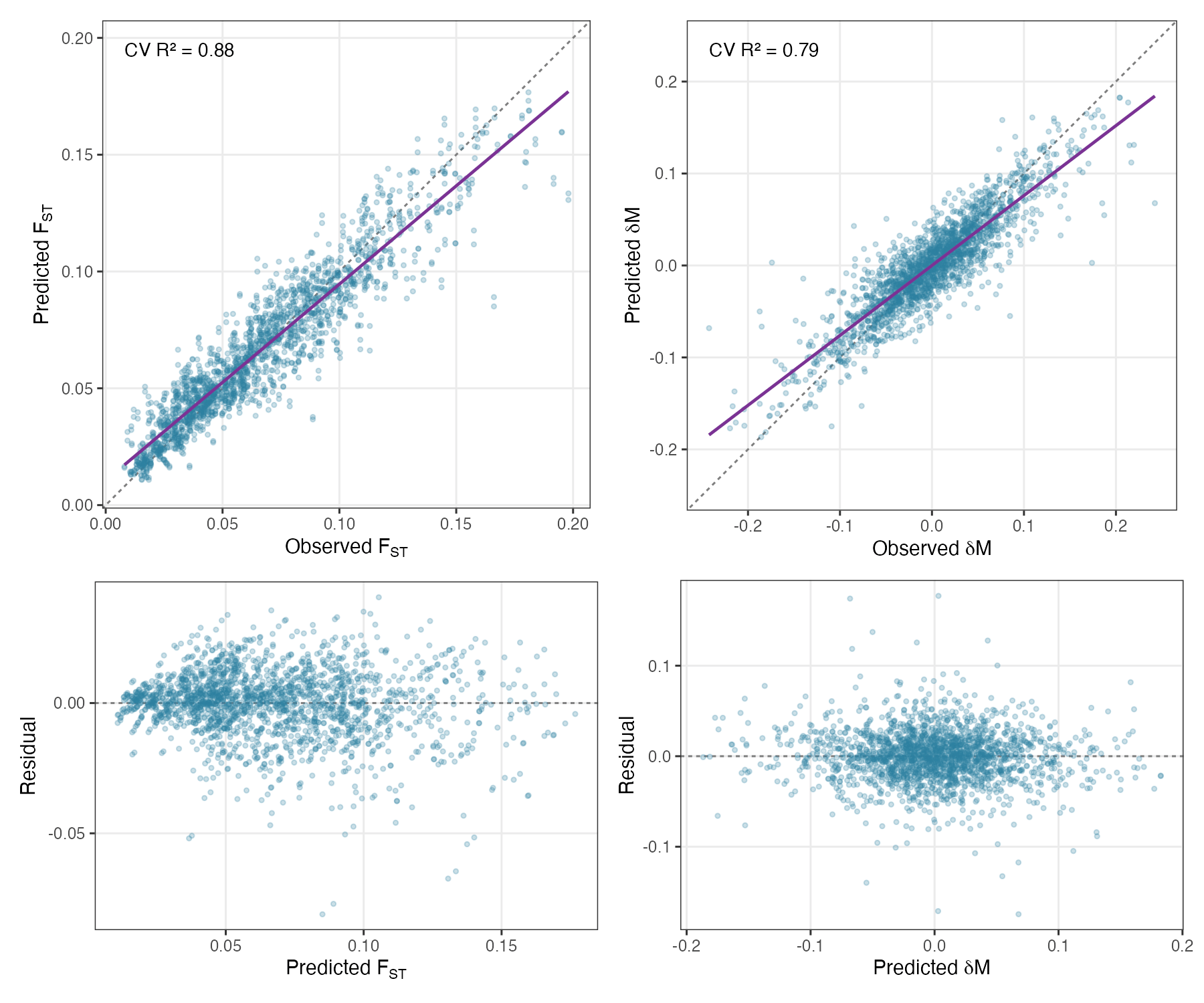
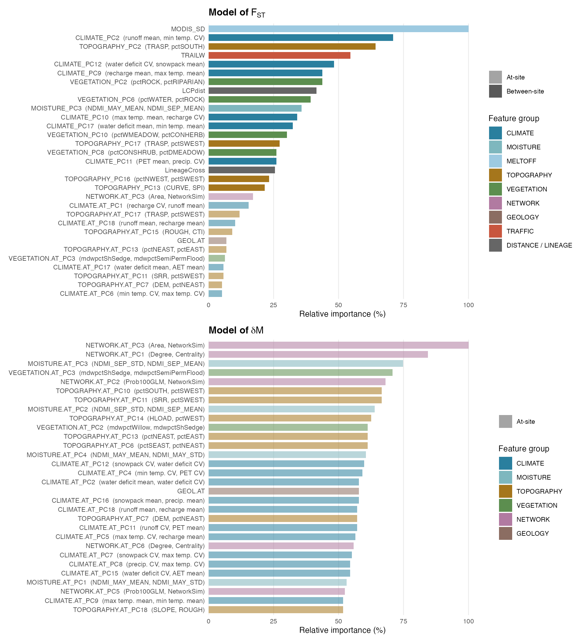
The two models emphasize different things. FST mostly reflects how connected two meadows are overall, and it leans on a few between-site features. δM reflects contrasts that favor movement in one direction, and many at-site features share the importance. Snowpack-related climate (meltoff timing variability, runoff, recharge) ranks high in both. For δM, contrasts in meadow area, number of neighboring meadows and breeding probability stand out, which echoes the hub and satellite structure we found within meadow neighborhoods.
Step 6. Forecasting connectivity under climate change
To forecast, we swap present climate for the 2070–2099 projections (CCSM4, RCP 8.5, a business-as-usual scenario) and project them onto the present-day PCA loadings, so the components keep their meaning. Every other feature stays as it is. The models then predict FST and δM for each directed pair, now and in the future.
fut <- setNames(clim_table[, paste0(GROUPS$CLIMATE, "_f")], GROUPS$CLIMATE)
Xf  <- X
Xf[, colnames(pca_climate$x)] <- predict(pca_climate, fut)   # same loadings as today
# (at-site climate is projected the same way)
now    <- predict(final$finalModel, X[, vars])
future <- predict(final$finalModel, Xf[, vars])
change <- future - now
To put these pairwise forecasts on a map, each pair’s value is spread over its LCC 0.05 corridor, scaled by the corridor weight so less likely routes count for less, and overlapping corridors are averaged cell by cell. For δM we also keep track of direction. Each pair contributes a vector from source to destination, reversed if δM is projected to drop, and the vectors are summed in every cell to give a net direction of change.
for (r in rows_of_this_pair) {
  s  <- sign(dm$change[r])
  dx <- xy[to, 1] - xy[from, 1]; dy <- xy[to, 2] - xy[from, 2]
  mag[on] <- mag[on] + w * abs(dm$change[r]); n[on] <- n[on] + 1
  vx[on]  <- vx[on] + w * dx * s;            vy[on] <- vy[on] + w * dy * s
}
# mean magnitude = mag / n; net bearing = atan2(vx, vy)
Finally, we treat the meadows as a network. Edges are weighted by how connected each pair is predicted to be (the maximum FST minus the predicted value), and eigenvector centrality shows how central each meadow is to park-wide gene flow, now and in the future.
library(igraph)
m[cbind(from, to)] <- max(c(fst_now, fst_future)) - fst_now
g <- graph_from_adjacency_matrix(m, mode = "max", weighted = TRUE)
centrality_now <- eigen_centrality(g)$vector
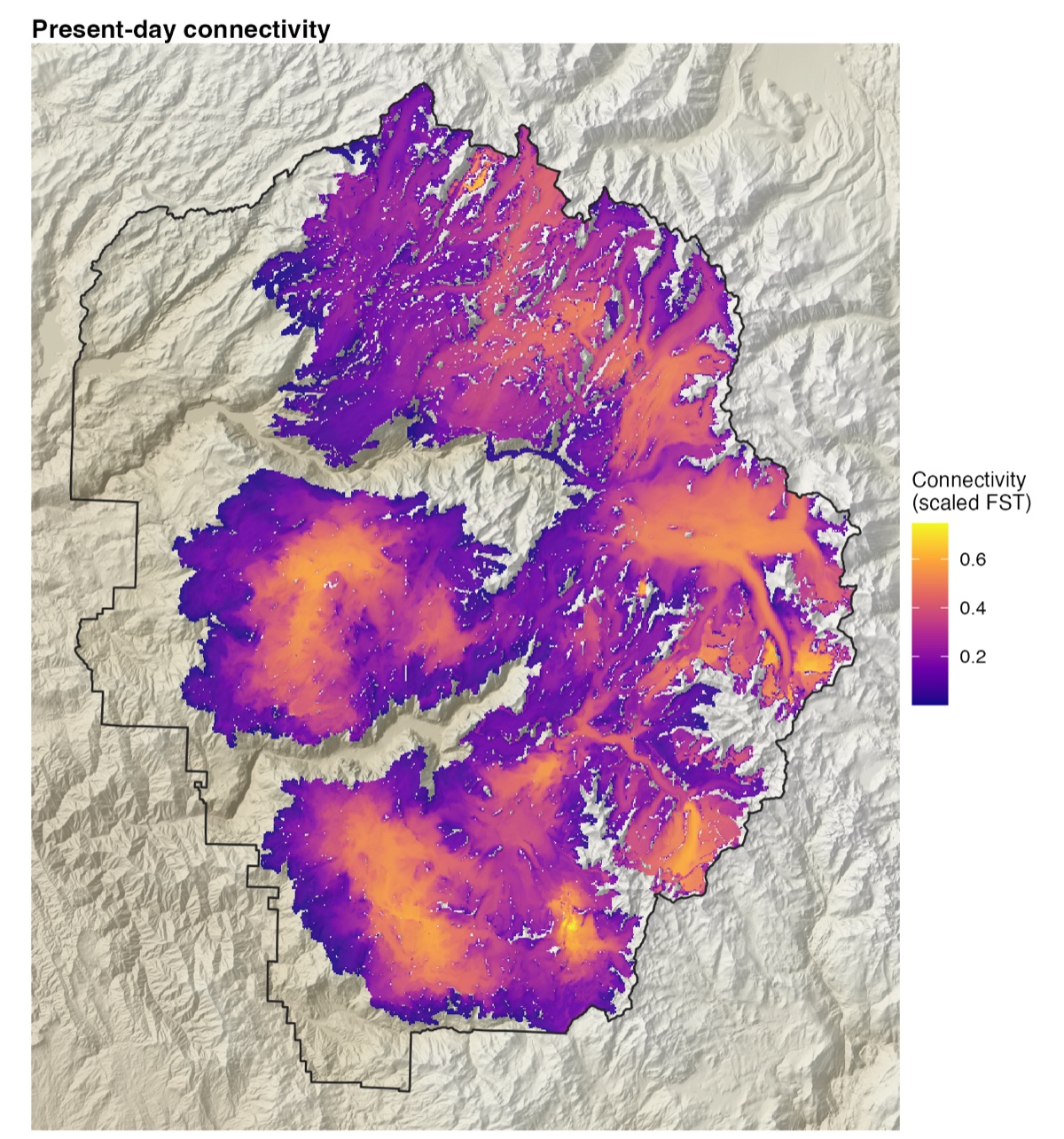
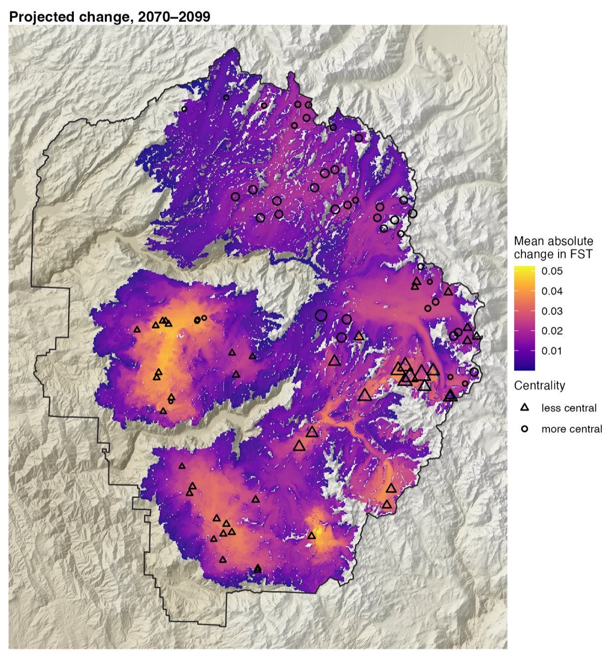
Connectivity now and in the future. Left: present-day connectivity, averaged over every corridor that covers a cell. Right: projected change in FST by 2070–2099, with meadows that become more central (circles) or less central (triangles) to the network.
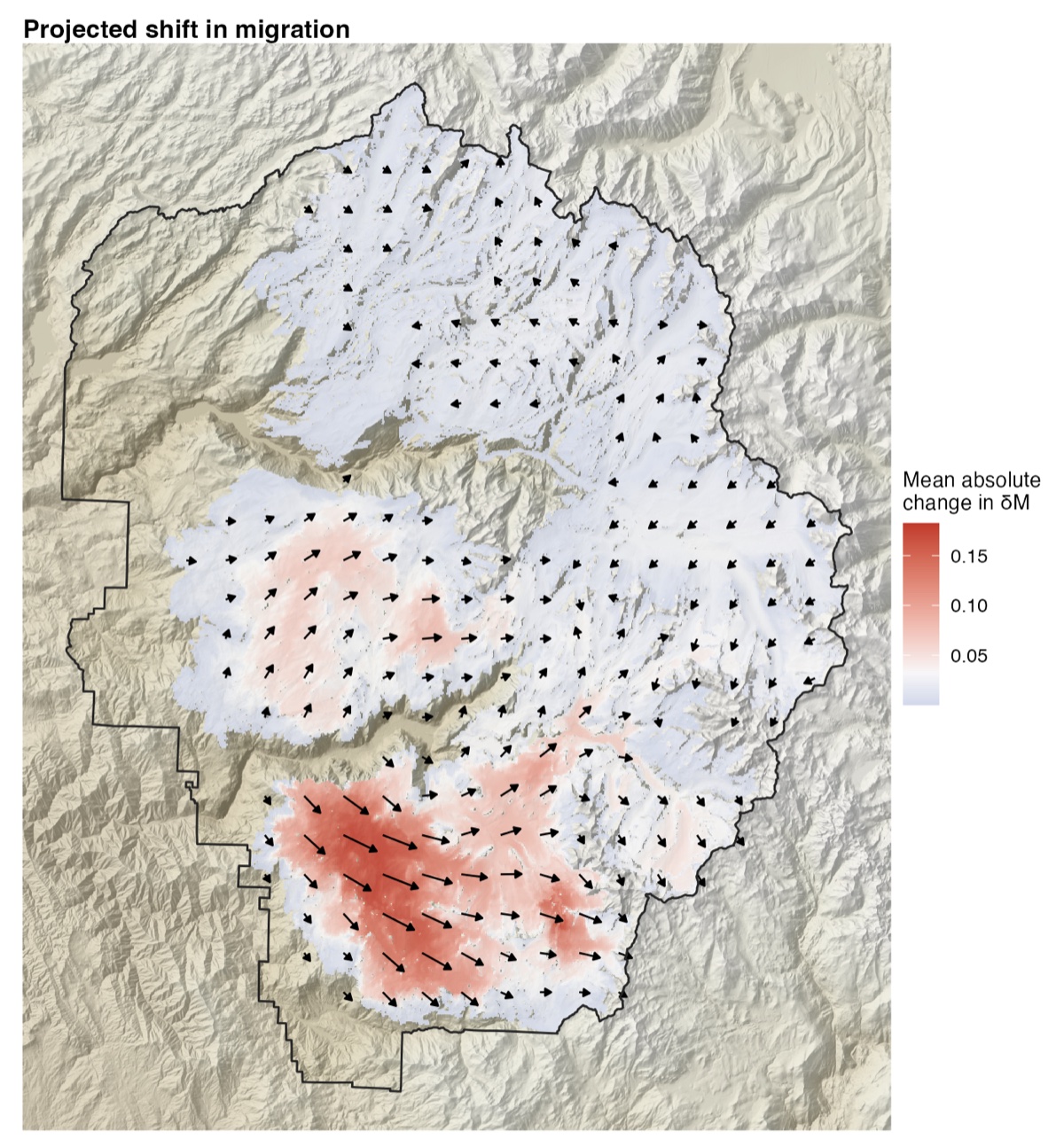
The connectivity surface shows regional corridors of high flow and pinch points where ridgelines, fire-prone low country or sparse meadow habitat cut across. The Y-North lineage, broken up by canyons, is poorly connected compared with the rest. Looking ahead, the biggest losses in connectivity fall on Y-West, Y-South and admixed areas in the south. Centrality moves from the south and west toward the north and east.
The δM forecast points the same way. Net movement runs from west to east, toward higher ground. Given the pinch points in the southern corridors, movement out of Y-South would go up the Middle Fork of the Merced River (north of the Clark Range) or up the South Fork straight into the Clark Range. Y-West has a single likely route up Tenaya Creek into the Tuolumne watershed. Smaller vectors inside Y-East and Y-North suggest some movement north as well. Taken together, the models predict a range shift toward higher elevation and latitude by 2100. These maps could help guide where to protect, or even assist, migration as lower meadows dry out.
Using this workflow for your own species
Nothing here is specific to toads. The approach suits any patch-limited species where you have pairwise genetic distances between discrete sites and a sense of what limits movement. A few things to keep in mind:
- The first model matters. Corridors come from a simple resistance model, so if that model is uninformed, the corridors will carry irrelevant landscape. Build it from features the literature already supports.
- Pre-modeling partials out some importance. Since paths were chosen on slope, topography ranks lower in the later models than it might otherwise. Read importance scores with that in mind.
- Direction is not in the importance scores. Tree ensembles say which features matter, not whether they raise or lower connectivity. Partial dependence plots help with that.
- Keep phylogeography in the model. Deep lineage splits add FST that has nothing to do with the current landscape. A lineage term soaks that up.
- Plan for scale. Accumulated cost surfaces and corridor rasters for a thousand pairs take time and disk space. Write them to disk once and run the extraction in parallel.
How to cite
- Maier PA, Vandergast AG, Ostoja SM, Aguilar A, Bohonak AJ (2022) Landscape genetics of a sub-alpine toad: climate change predicted to induce upward range shifts via asymmetrical migration corridors. Heredity 129:257–272. doi:10.1038/s41437-022-00561-x. Data: doi:10.5061/dryad.xsj3tx99h
Related work
- Maier PA, Vandergast AG, Ostoja SM, Aguilar A, Bohonak AJ (2022) Gene pool boundaries for the Yosemite toad (Anaxyrus canorus) reveal asymmetrical migration within meadow neighborhoods. Frontiers in Conservation Science 3:851676. doi:10.3389/fcosc.2022.851676
- Maier PA, Vandergast AG (2024) Yosemite toad (Anaxyrus canorus) transcriptome reveals interplay between speciation genes and adaptive introgression. Molecular Ecology 33:e17317. doi:10.1111/mec.17317
- Maier PA, Vandergast AG, Ostoja SM, Aguilar A, Bohonak AJ (2019) Pleistocene glacial cycles drove lineage diversification and fusion in the Yosemite toad (Anaxyrus canorus). Evolution 73:2476–2496. doi:10.1111/evo.13868
- Peterman WE (2018) ResistanceGA: an R package for the optimization of resistance surfaces using genetic algorithms. Methods in Ecology and Evolution 9:1638–1647.
- Sundqvist L, Keenan K, Zackrisson M, Prodöhl P, Kleinhans D (2016) Directional genetic differentiation and relative migration. Ecology and Evolution 6:3461–3475.
- van Etten J (2017) R package gdistance: distances and routes on geographical grids. Journal of Statistical Software 76:1–21.
- Quinlan JR (1993) Combining instance-based and model-based learning. Proceedings of the Tenth International Conference on Machine Learning, 236–243.
- Berlow EL, Knapp RA, Ostoja SM et al. (2013) A network extension of species occupancy models in a patchy environment applied to the Yosemite toad (Anaxyrus canorus). PLoS ONE 8:e72200.